The Interpolation Search Algorithm with Python

The interpolation searching algorithm is an improved version of the binary search algorithm. It performs very efficiently when there are uniformly distributed elements in the sorted list. In a binary search, we always start searching from the middle of the list, whereas in the interpolation search we determine the starting position depending on the item to be searched. In the interpolation search algorithm, the starting search position is most likely to be the closest to the start or end of the list depending on the search item. If the search item is near to the first element in the list, then the starting search position is likely to be near the start of the list.

The interpolation search is another variant of the binary search algorithm that is quite similar to how humans perform the search on any list of items. It is based on trying to make a good guess of the index position where a search item is likely to be found in a sorted list of items. It works in a similar way to the binary search algorithm except for the method to determine the splitting criteria to divide the data in order to reduce the number of comparisons. In the case of an interpolation search, we divide the data using the following formula:

mid_point = lower_bound_index + \
    (upper_bound_index - lower_bound_index) * \
    (search_value - input_list[lower_bound_index]) // \
    (input_list[upper_bound_index] - input_list[lower_bound_index])

In the preceding formula, the lower_bound_index variable is the lower-bound index, which is the index of the smallest value in the input_list list, denoting the index position of the lowest value in the list. The input_list[lower_bound_index] and input_list[upper_bound_index] variables are the lowest and highest values respectively in the list. The search_value variable contains the value of the item that is to be searched.

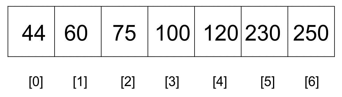
Let's consider an example to understand how the interpolation searching algorithm works using the following list of 7 items:

To find 120, we know that we should look at the right-hand portion of the list. Our initial treatment of binary search would typically examine the middle element first in order to determine if it matches the search term.

A more human-like method would be to pick a middle element in such a way as to not only split the array in half but to get as close as possible to the search term. The middle position was calculated using the following rule:

mid_point = (index_of_first_element + index_of_last_element) // 2

We shall replace this formula with a better one that brings us closer to the search term in the case of the interpolation search algorithm. The mid_point will receive the return value of the nearest_mid function, which is computed using the following method:

def nearest_mid(input_list, lower_bound_index, upper_bound_index, search_value):
    return lower_bound_index + \
        (upper_bound_index - lower_bound_index) * \
        (search_value - input_list[lower_bound_index]) // \
        (input_list[upper_bound_index] - input_list[lower_bound_index])

The nearest_mid function takes, as arguments, the lists on which to perform the search. The lower_bound_index and upper_bound_index parameters represent the bounds in the list within which we are hoping to find the search term. Furthermore, search_value represents the value being searched for.

Given our search list, 44, 60, 75, 100, 120, 230, and 250, nearest_mid will be computed with the following values:

lower_bound_index = 0
upper_bound_index = 6
input_list[upper_bound_index] = 250
input_list[lower_bound_index] = 44
search_value = 230

Let's compute the mid_point value:

mid_point = 0 + (6-0) * (230-44) // (250-44)
          = 5

It can now be seen that the mid_point value will receive the value 5. So, in the case of an interpolation search, the algorithm will start searching from the index position 5, which is the index of the location of our search term. Thus, the item to be searched will be found in the first comparison, whereas in the case of a binary search, we would have chosen the position of 100 as mid_point, which would have required another run of the algorithm.

A more visual illustration of how a typical binary search differs from an interpolation is given as follows. In a typical binary search, it finds the midpoint that looks like it's in the middle of the list:

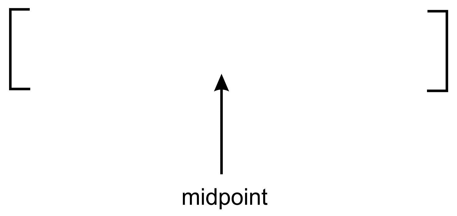
One can see that the midpoint is actually standing approximately in the middle of the preceding list. This is as a result of dividing the list by two.

In the case of an interpolation search, on the other hand, the midpoint is moved to the most likely position where the item can be matched:

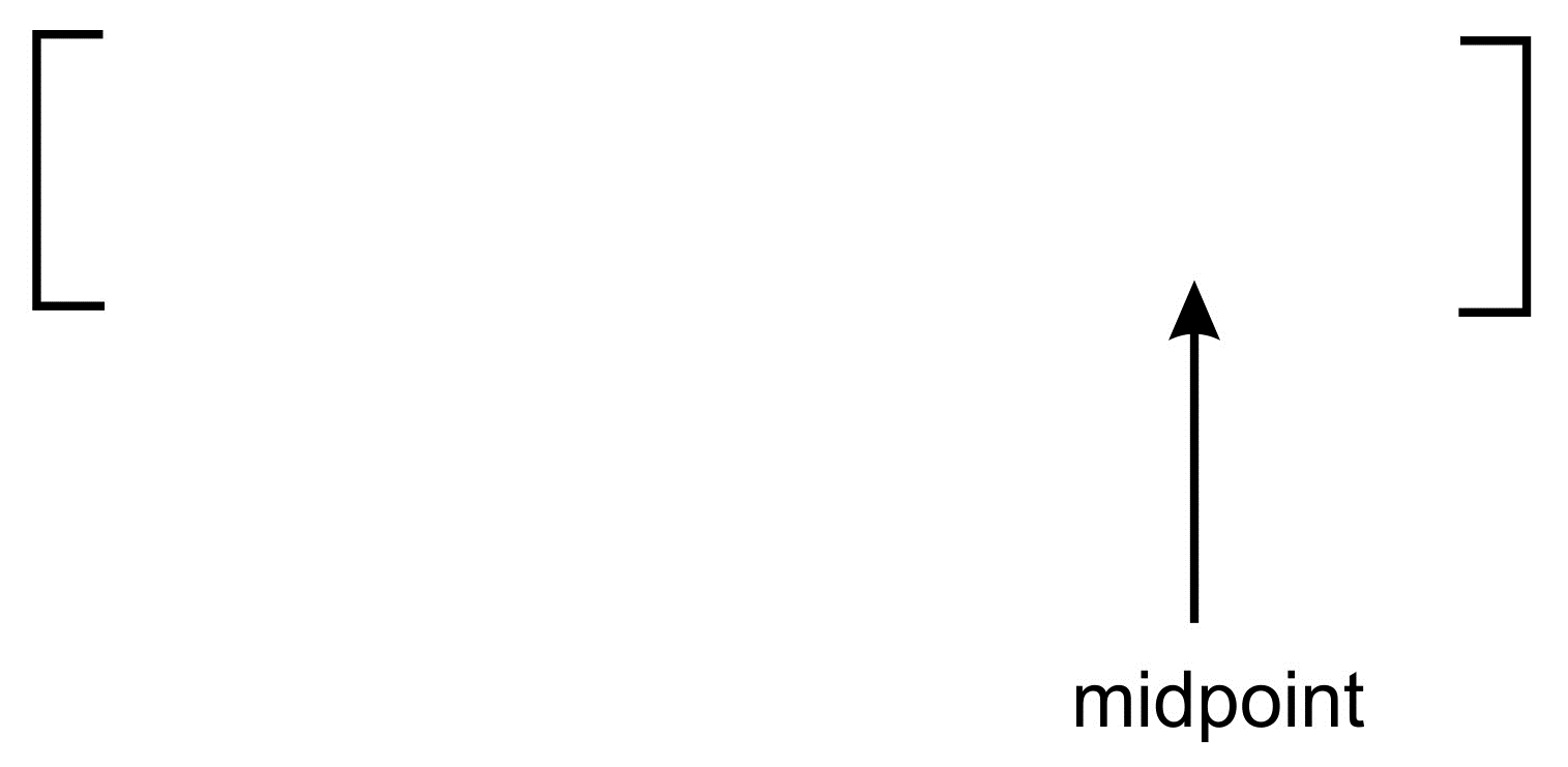
In an interpolation search, the midpoint is generally more to the left or right. This is caused by the effect of the multiplier being used when dividing to obtain the midpoint. In the preceding diagram, our midpoint has been skewed to the right.

The implementation of the interpolation algorithm remains the same as that of the binary search except for the way we compute the midpoint.

Here, we provide the implementation of the interpolation search algorithm, as shown in the following code:

def interpolation_search(ordered_list, term):

    size_of_list = len(ordered_list) - 1

    index_of_first_element = 0
    index_of_last_element = size_of_list

    while index_of_first_element <= index_of_last_element:
        mid_point = nearest_mid(ordered_list, index_of_first_element, index_of_last_element, term)

        if mid_point > index_of_last_element or mid_point < index_of_first_element:
            return None

        if ordered_list[mid_point] == term:
            return mid_point

        if term > ordered_list[mid_point]:
            index_of_first_element = mid_point + 1
        else:
            index_of_last_element = mid_point - 1

    if index_of_first_element > index_of_last_element:
        return None

The nearest_mid function makes use of a multiplication operation. This can produce values that are greater than upper_bound_index or lower than lower_bound_index. When this occurs, it means the search term, term, is not in the list. None is, therefore, returned to represent this.

So, what happens when ordered_list[mid_point] does not equal the search term? Well, we must now readjust index_of_first_element and index_of_last_element so that the algorithm will focus on the part of the array that is likely to contain the search term.

if term > ordered_list[mid_point]:
    index_of_first_element = mid_point + 1

If the search term is greater than the value stored at ordered_list[mid_point], then we only adjust the index_of_first_element variable to point to the mid_point + 1 index.

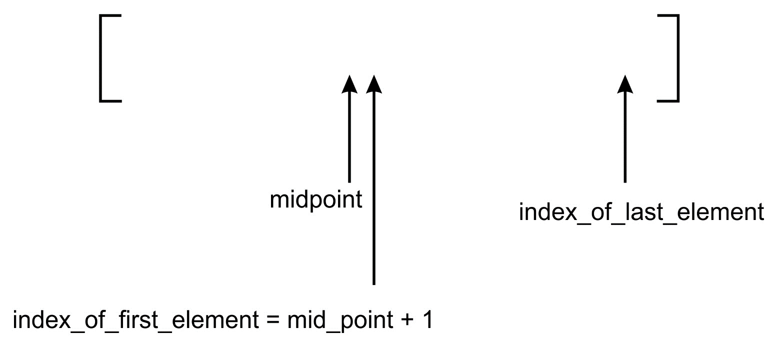
The following diagram shows how the adjustment occurs. The index_of_first_element is adjusted and pointed to the mid_point + 1 index:

On the other hand, if the search term is less than the value stored at ordered_list[mid_point], then we only adjust the index_of_last_element variable to point to the index mid_point - 1. This logic is captured in the else part of the if statement index_of_last_element = mid_point - 1:

The diagram shows the effect of the recalculation of index_of_last_element on the position of the midpoint.

Let's use a more practical example to understand the inner workings of both the binary search and interpolation algorithms.

Consider for example the following list of elements:

[ 2, 4, 5, 12, 43, 54, 60, 77]

At index 0, the value 2 is stored, and at index 7, the value 77 is stored. Now, assume that we want to find the element 2 in the list. How will the two different algorithms go about it?

If we pass this list to the interpolation search function, then the nearest_mid function will return a value equal to 0 using the formula of mid_point computation which is as follows:

mid_point = 0 + (7-0) * (2-2) // (77-2)
          = 0

As we get the mid_point value 0, we start the interpolation search with the value at index 0. Just with one comparison, we have found the search term.

On the other hand, the binary search algorithm needs three comparisons to arrive at the search term, as illustrated in the following diagram:

The first mid_point value calculated is 3. The second mid_point value is 1 and the last mid_point value where the search term is found is 0.

Therefore, it is clear that the interpolation search algorithm performs better than binary search in most cases.

The binary search and interpolation search algorithms are better in performance compared to both ordered and unordered linear search functions. Because of the sequential probing of elements in the list to find the search term, ordered and unordered linear searches have a time complexity of O(n). This gives a very poor performance when the list is large.

The binary search operation, on the other hand, slices the list in two anytime a search is attempted. On each iteration, we approach the search term much faster than in a linear strategy. The time complexity yields O(log n). Despite the speed gain in using a binary search, the main disadvantage of it is that it cannot be applied on an unsorted list of items, neither is it advised to be used for a list of small size due to an overhead of sorting.

The ability to get to the portion of the list that holds a search term determines, to a large extent, how well a search algorithm will perform. In the interpolation search algorithm, the midpoint is computed in such a way that it gives a higher probability of obtaining our search term faster. The average-case time complexity of the interpolation search is O(log(log n)), whereas the worst-case time complexity of the interpolation search algorithm is O(n). This shows that interpolation search is better than binary search and provides faster searching in most cases.

If you found this article interesting, you can explore Hands-On Data Structures and Algorithms with Python to learn to implement complex data structures and algorithms using Python. Hands-On Data Structures and Algorithms with Python teaches you the essential Python data structures and the most common algorithms for building easy and maintainable applications.